
The Rational method, which was formulated more than a century ago, remains a prevalent approach for modeling urban watersheds, particularly for areas that are smaller than approximately 200 acres. Although numerous versions of the Rational method exist, Stormwater Studio employs the widely adopted variant known as the Standard Rational method.
Standard Rational
The Standard Rational method computes the peak discharge as determined by the well-known Rational formula.
Where:
Qp = peak discharge, cfs (cms)
k = 1 English (0.00278 Metric)
C = runoff coefficient
A = basin area, acres (hectares)
i = intensity, in/hr (mm/hr)
Cf = frequency correction factor where C x Cf <= 1.0
The rainfall intensity is computed by one of the following equations:
FHA Equation
Where:
B, D and E are constants
Tc = time of concentration in minutes subject to the Minimum Tc
Third Degree Polynomial Equation
Where:
I = rainfall intensity in in/hr (mm/hr)
X = Ln(time duration in minutes)
A = coefficient
B = coefficient
C = coefficient
D = coefficient
Appropriate values for X are 8 to 180 minutes subject to the Minimum Tc.
The B,D and E constants can be pre-computed by the program, or as manually entered, and are based on your geographic location. Polynomial coefficients can be directly entered in to software as well.
Calculation Procedure for Time of Concentration, Tc, and Flows
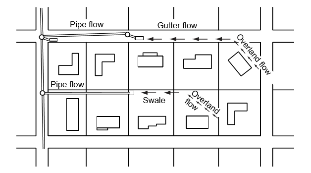
The software computes flows starting from the most upstream Line and proceeds downstream. The Q’s are evaluated at each junction and are based on the Tc at eaach junction. The time of concentration is the time required for water to flow from the remotest point of the drainage area to the current junction. The program computes Tc at each inlet or junction by choosing the greatest of the following:
- The time of concentration of the upstream Line plus the time of flow through the Line from the upstream run.
- The time of concentration as above for any other connecting Line(s).
- The Inlet Time of the Line under consideration.
For the most upstream run, the time of concentration is the Inlet Time. For all succeeding lines, the time of concentration is computed as the largest value of the three items above.
When calculating flows for downstream lines, Stormwater Studio employs a total CxA, which includes the CA for the specific Line in question, the CA for the next upstream Line, and the CA for subsequent upstream Lines, continuing in this manner. This approach ensures that all drainage areas are accounted for in contributing flow to the catchment of interest. It is important to note that the calculated Qs at each point within the system may not algebraically total the upstream flows.
Rational Method Anomalies
As mentioned earlier, the flow path with the longest time of concentration to the point of interest in your storm sewer system typically determines the storm duration used in selecting the intensity value in the Rational method. However, there are some important exceptions that you should be aware of.
One such exception can be observed when reviewing your Standard Report and finding an extremely long System Tc. This is commonly seen in long, narrow wooded lots with a small runoff coefficient that will remain undeveloped but still need to be accounted for in the new development. When including this particular area in the runoff calculation, the resulting long time of concentration will lead to smaller Peak Qs, resulting in pipes that are designed too small to handle the internal flows from a shorter duration storm. To address this issue, adjustments will need to be made by simply disregarding those specific areas (or a portion of them) where the flow time is too slow to contribute to the peak discharge.
Here’s what to do and how to do it:
There are generally two scenarios:
1. A highly impervious section exists at the most downstream area of an inlet’s watershed and the rogue upstream area flows through the lower impervious area. Two separate calculations should be made to find the area – either the Total or the Impervious – which produces the highest Q.

• First, calculate the Peak Q from the total drainage area with its weighted C value and the intensity associated with the longest time of concentration, Tc. (Stormwater Studio has probably already done this for you during its normal calculation routine.)
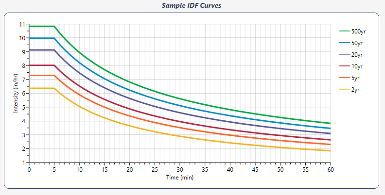
• Secondly, calculate the Peak Q using only the smaller, Impervious Area, its C value and intensity associated with its shorter Tc. (Pull from the IDF curves.)
Compare the two and only use the drainage area, C and Tc that produces the highest Peak Q. This typically will be the smaller area. Disregard the larger, slower area.
2. A smaller, less pervious, area is tributary to the larger primary drainage area. When this scenario occurs, two sets of calculations should also be made.
• First, calculate the Peak Q from the total drainage area with its weighted C value and the intensity associated with the longest time of concentration, Tc. (Stormwater Studio has probably already done this for you during its normal calculation routine.)
• Secondly, prorate the larger drainage area. We need to learn how much discharge from the larger, slower area is contributing at the same time the peak from the smaller less pervious tributary area is occurring. For example, if the smaller tributary area has a Tc of 10 minutes, how much area from the larger, slower area, is contributing after 10 minutes?
Prorate it. We’ll call that prorated area, Ap. It’s the most downstream fractional part of the larger area that will contribute to the flow during the time of concentration associated with the smaller, less pervious area.
Ap = A (Tc1 / Tc2)
Where:
Ap = Prorated area
A = Area of the larger primary area
Tc1 = Time of concentration of the smaller tributary area
Tc2 = Time of concentration associated with the larger area
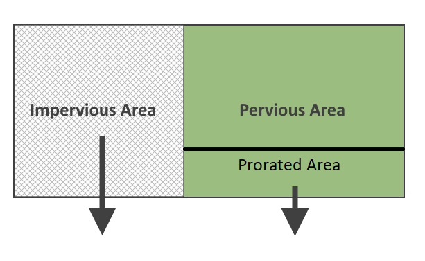
The C value to be used in this computation should be the weighted C value that results from combining C values of the smaller less pervious tributary area and the prorated area Ap. The area to be used would be the area of the smaller impervious area plus Ap. Your composite Area, C inputs would look similar to the inputs shown below. You would use the shorter Time of Concentration, Tc1.

Please keep in mind that this prorated method assumes a linear relationship between Tc and Area, i.e., the overland travel time is basically constant as it travels downstream.
Tc by TR55
In addition to manual entry, Stormwater Studio can compute Time of Concentration using TR55. With TR55, Tc is broken into 3-components or segments. The final Tc is the sum total of the three components.
- Sheet Flow
- Shallow Concentrated Flow
- Channel Flow
Tc = TSheet + TShallow + TChannel
Sheet Flow Time
Flow over plane surfaces and typically ranges between 125 to 150 feet (40 to 45 meters).

Where:
n = Manning’s roughness coefficient
L = Flow Length (must be <= 100 ft (30 m) per WinTR55)
P2 = Two-year 24-hr rainfall, inches (mm). If this field is set to zero, the software will attempt to compute the value from your IDF curves using the 2-year curve at 1,440 minutes.
S = Land Slope, ft/ft (m/m) – Entered as % in the program
Shallow Concentrated Flow Time
After about 100 feet, sheet flow becomes shallow concentrated flow. The computed Average Velocity described below is based on the solution of Manning’s equation with different assumptions for n (Manning’s roughness coefficient) and r (hydraulic radius, ft). Per TR55, for for paved areas, n is 0.025 and r is 0.2; unpaved areas, n is 0.05 and r is 0.4.

Where:
L = Flow Length, ft (m)
V = Average velocity, ft/s (m/s) and

Where:
Cp = 20.3282 paved surfaces
Cp = 16.1345 unpaved surfaces
S = Watercourse slope, ft/ft (m/m)
Channel Flow Time
Occurs within channels, swales, ditches, streams or even piped systems. Manning’s equation is used to compute velocity.

Where:
L = Flow length, ft (m)
V = Average velocity, ft/s (m/s) and

Where:
V = Average velocity, ft/s (m/s)
R = Hydraulic radius, ft (m) = a/wp
S = Channel slope, ft/ft (m/m) – Entered as % in the program
n = Manning’s roughness coefficient