One of the great features of Hydrology Studio is its flexibility. You can add data to any hydrograph at any time. In other words, you can build out the entire watershed model as we did in the Part I of this tutorial first, and then add data; or you can add the associated data as you work downstream. There’s no particular order you need to follow. Preferably upstream to downstream when there will be junctions or routings.
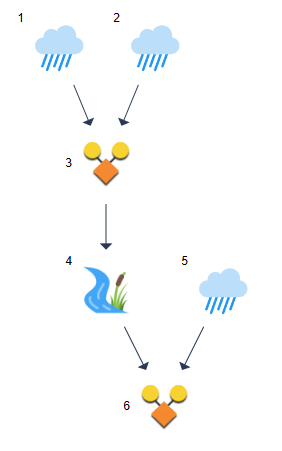
Here is the model we built in Part I of this tutorial. To recap: runoff hydrographs 1 and 2 met at a confluence so they were combined to form a Junction, Hydrograph No. 3. This hydrograph was then routed through a channel “Reach”, Hydrograph No. 4. This hydrograph was then combined with another runoff hydrograph, Hydrograph 5, to create the final downstream Hydrograph No. 6.
 Now we can add data to each hydrograph, one-by-one.
As you may have already noticed, when clicking on a hydrograph icon, the Input Window changes to correspond to the selected hydrograph. To demonstrate, click on Hydrograph 1. The Input Window appears as follows:

Name Prefix is cosmetic only. Use these to add Pre or Post to your Hydrograph Names.
Just fill in the blanks, click [Compute] and Hydrology Studio creates your finished hydrograph. Use this procedure for all hydrographs in your basin models.
Hydrographs 1 & 2 – NRCS Runoff
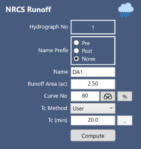
Input Data for Hydrograph No. 1

Input Data for Hydrograph No. 2
Hydrograph 3 – Junction
Click on Hydrograph number 3, Junction. Enter “Confluence” in the name field and click [Compute]. Notice the hydrographs (DA1 and DA2) to be added are already chosen.
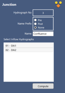
Input Data for Hydrograph No. 3
Hydrograph 4 – Channel Reach
Click on the Reach icon, Hydrograph 4, and enter the following data:
Data for Hydrograph No. 4
Hydrograph 5 – SCS Runoff
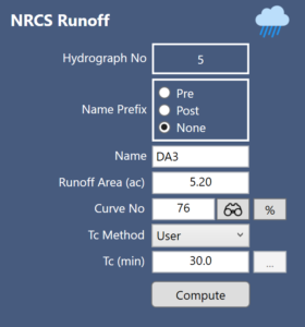
Data for Hydrograph No. 5
Hydrograph 6 – Junction
Click on Hydrograph number 6, Junction. Enter “Inflow to Channel (or Pond)” in the name field and click [Compute].
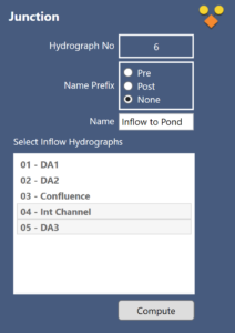
Data for Hydrograph No. 6
Data Entry is Complete
Now lets take a look at the Charts tab by clicking on Charts.
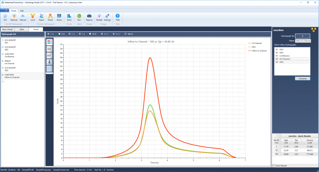
Select any hydrograph on the List box to the left to view its corresponding chart.
Viewing Different Return Periods
Note that Hydrology Studio computes hydrographs for all “Active” return periods at once. The frequency selector bar across the top allows you to choose which one to view. Just select one of the radio buttons and that return period will be displayed.
Active Return Periods are set at the Rainfall Wizard window. See, Choose Design Storm & Return Periods. There you can select which return periods the program will always use. The frequency shown below indicates that the 2, 10 and 100-years are “Active”. All other frequencies have been set as “Inactive” and thus disabled.

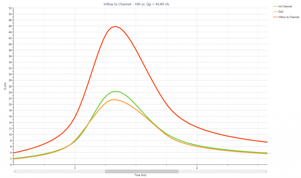
How to Zoom
Any chart in this software can be zoomed by simply dragging a rectangle from the upper left to the lower right of a desired viewport. Double-click the chart to return to full extents.
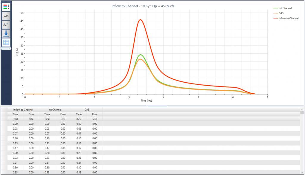
View the Numerical Chart
You can include a table with the selected hydrographs numerical values by clicking on the Grid button on the side tool bar. The values in this table can be included in the formal printed reports but you can also export this exact table to a .csv spreadsheet file by right-clicking on the table and selecting, “Export this grid…”.

Conclusion
Hopefully you are now equipped with the know-how to create and model a watershed, no matter how large or small or complex. At this point you’re ready to print reports. Hydrology Studio offers many different types and styles including options to include a Table of Contents. Please see, Printing Reports for more information.