Learn how to create a pre- and post-development drainage study with a detention pond design using Hydrology Studio. By following this easy example, you’ll be able to complete similar projects quickly and efficiently. Plus, your designs will be top-notch!
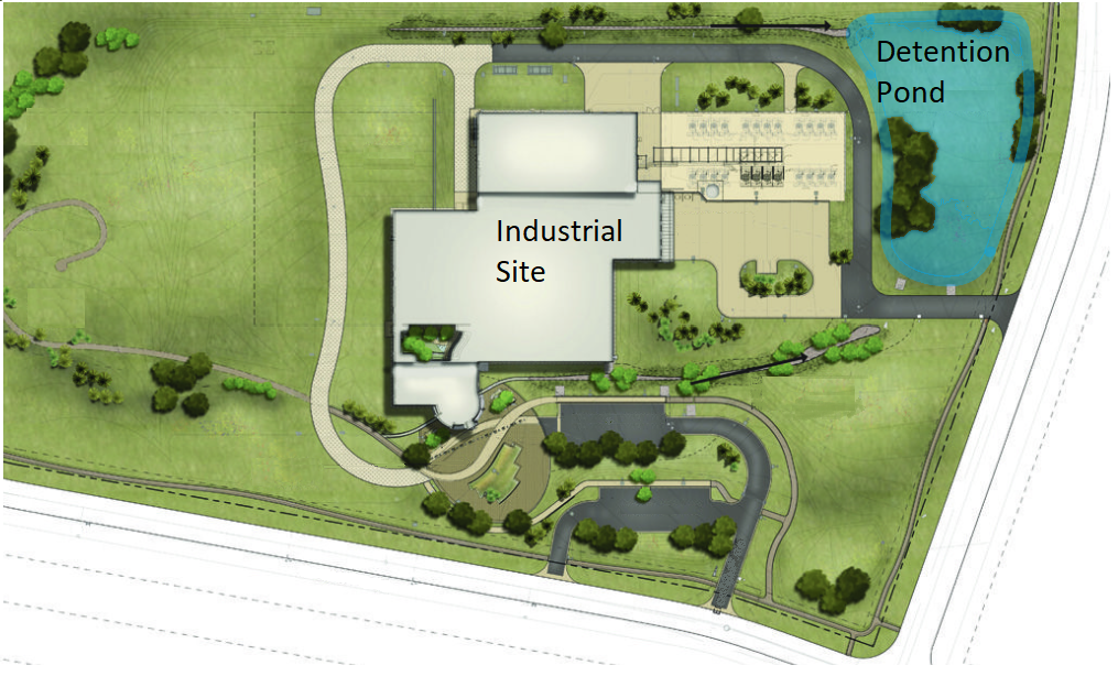
You’ll start with a 10-acre undeveloped site, “Meadow in good condition”. The site will be transformed into an industrial complex. Our task is to attenuate the peak runoff rate produced by the development to that of the pre-developed condition for the 2, 10 and 100-year return periods.
We are going to use the SCS (NRCS) hydrograph method using an IDF based synthetic “Balanced Storm” 6-hr duration for producing the runoff hydrographs. This design storm and IDF curves are already installed as defaults that come with your software, out-of-the-box. So there’s nothing you’ll need to do with that if you plan to follow along.
You can, however, use any other design storm such as one of the NRCS 24-hour distributions if you like. The procedure is the same.
Here are the pre- and post-developed Curve Numbers and Tc’s.
Pre/Post Data Inputs
| Scenario | NRCS - 6-hr Synthetic "Balanced" Design Storm | |
|---|---|---|
| Area (ac) | 10.00 | |
| Pre-dev | CN | 71 |
| Tc (min) | 30 | |
| Post-dev | CN | 91 |
| Tc (min) | 12 |
In a nutshell the procedure follows these steps:
- Create the pre-developed hydrograph
- Create the post-developed hydrograph
- Design a detention pond using a simple 3-Step process
- Print reports
Create the Basin Model
If you have read the tutorial on Building a Watershed Model this will be very easy.
Add the Pre-developed Hydrograph to Your Model
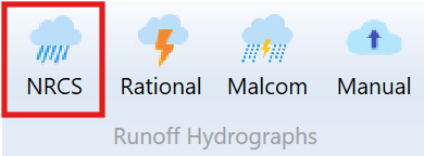
On the Basin Model tab, click the [NRCS] button on the top ribbon menu. This will automatically add an NRCS hydrograph icon to the model and will represent our pre-developed hydrograph.
Add the Post-developed Hydrograph to Your Model
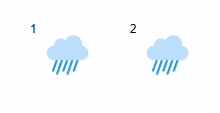
Click the [NRCS] button again. This will automatically add a second NRCS hydrograph icon to the model and will represent our post-developed hydrograph.
Your model should now look like this:
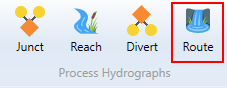
Add the Pond Route Hydrograph to Your Model
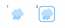
Next you’ll add the Pond Route hydrograph assigning Hydrograph 2 (Post) as its Inflow hydrograph. To do this, select Hydrograph 2 by clicking on it with your mouse (you’ll see a blue rectangle around it) and then click the Route button on the top ribbon menu.
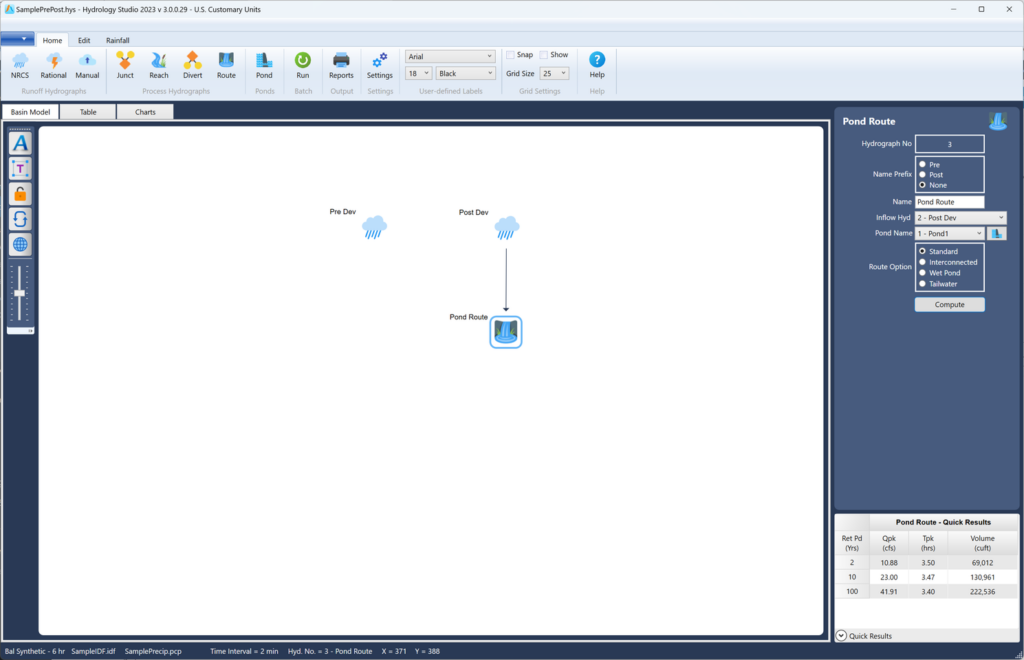
Your model should now look like the following:
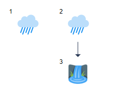
Hydrograph 1 is the predeveloped; Hydrograph 2 is the post-developed; and Hydrograph 3 is the detention pond routing that attenuates Hydrograph 2 back to the pre-developed condition.
Your Basin Model is Complete
That is all that’s needed to build a pre/post development model. Simply create runoff hydrographs representing the pre- and post-development conditions and then add the pond routing hydrograph. Remember, the pond routed hydrograph icon represents a “Hydrograph” exiting the pond. Not the detention pond itself. We’ll add the pond later. The Basin Model only contains actual “hydrographs”.
In more complex watersheds, your runoff hydrographs could consist of multiple sub-basins added together using the [Junct] function, creating a single, combined hydrograph.
Add the Data
At this point your model is only a schematic and contains no data, i.e., drainage areas, curve numbers, Tc, etc. Now we will add the data for the runoff hydrographs.
Pre-developed Hydrograph
Select Hydrograph 1 by clicking on it. This will provide a data input box on the right where you can enter the corresponding data.
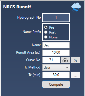
Enter the data as shown above and click the [Compute] button.
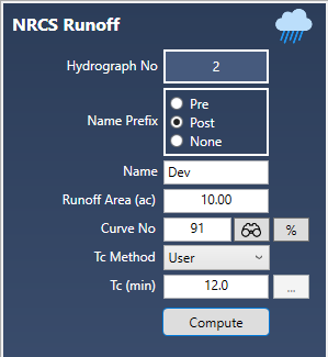
Post-developed Hydrograph
Select Hydrograph number 2 and enter its data as shown below and click [Compute].
Now lets take a look at the Charts by clicking on Charts tab at the upper left.
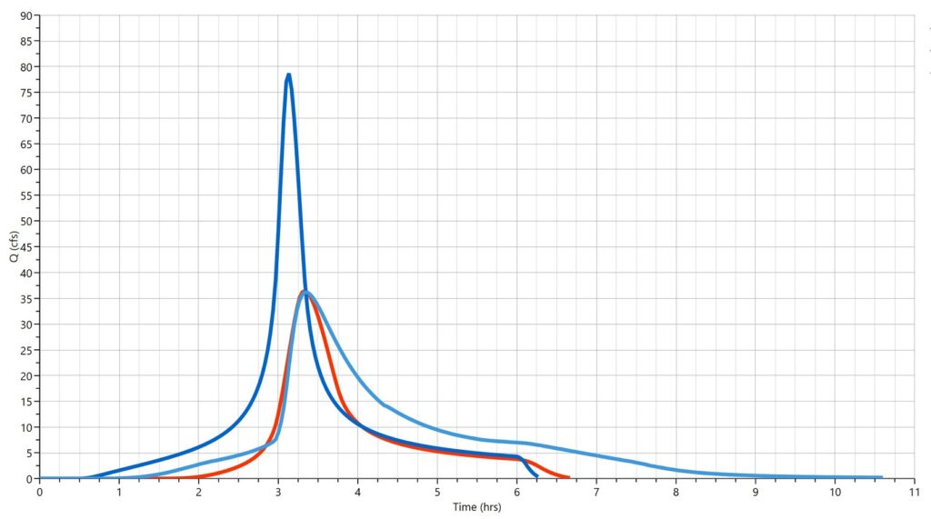
Click on Hydrographs 1 & 2 on the list box to the left while holding down your [Shift] key. This will plot both selected hydrographs. Click on the 100-yr radio button above the graph to view the 100-year event.
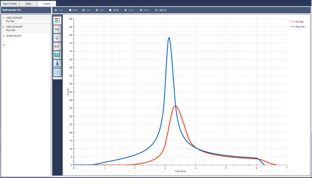
As you can see, the post-development increased the Peak runoff rate to 79 cfs from 36 cfs in its natural state. Our goal now is to design a detention pond that will produce an outflow hydrograph that looks similar to the pre-developed (red) hydrograph for the 2, 10 and 100-year events.
Design Your Detention Pond
Start by clicking on the Basin Model tab and selecting Hydrograph number 3. The input box will appear. Enter data as shown below but DO NOT click [Compute] yet.
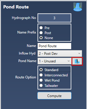
Now click the Pond button (in red box) to open the Pond Designer. (You can also open the Pond Designer by clicking on the [Pond] button from the top Ribbon menu.) The Pond Designer will look like this:
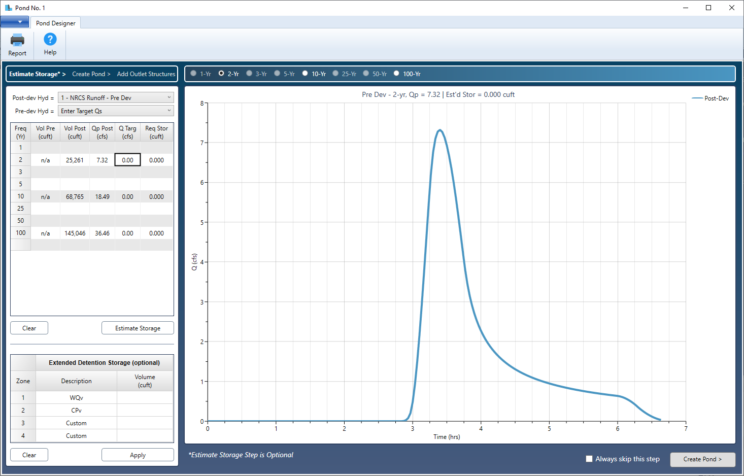
The Pond Designer is setup in a wizard-like way and will guide you from start to finish using just three steps. We’ll walk through them one-by-one.
- Step 1 – Estimate Storage. This step provides you with an estimate of how large your pond should be. It requires a specified Inflow hydrograph and Target outflows.
- Step 2 – Create Pond. This steps helps you build the physical pond that matches the estimated storage from Step 1.
- Step 3 – Add Outlet Structures. The final step is where you add outlet devices like culverts, orifices, weirs, etc. It also allows you to perform intermediate trial routings so that you can arrive at a perfect final design, quickly.
Step 1 – Estimate Storage
Start by selecting the Pre and Post Hydrographs from the drop-down list boxes as shown below. (The Post-dev is Hydrograph 2; the Pre-dev is Hydrograph 1) and clicking [Estimate Storage].
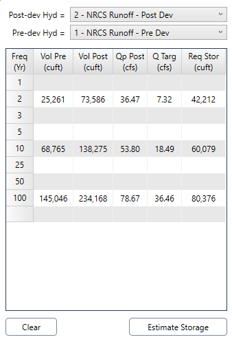
Notice the values at the lower right corner of this output table. It shows that you’ll need a pond with approximately 80,376 cubic feet of available storage in order to meet the pre-developed Target Qs. You’ll also notice a chart that plots the Pre and Post-developed hydrographs as well as the Target hydrograph. The blue shaded area represents the Estimated Storage. Note that this estimate will be 10 to 15 percent accurate (+/-) when using NRCS. It’s a pretty good estimate to use as a guide to your final designs.
Step 2 – Create the Pond
Once we have determined the amount of storage we’re going to need, we can use this step to actually create a pond that meets that storage. Click the [Create Pond] button on the lower right of this window to move to Step 2 where we will define the actual pond.
Selecting a Storage Type
The software allows you to choose a variety of methods for describing the physical properties of your pond. You can set it up by describing:
- Elevation contours
- Trapezoidal shapes
- Manually entering in known incremental volumes
- Underground Storage Chambers
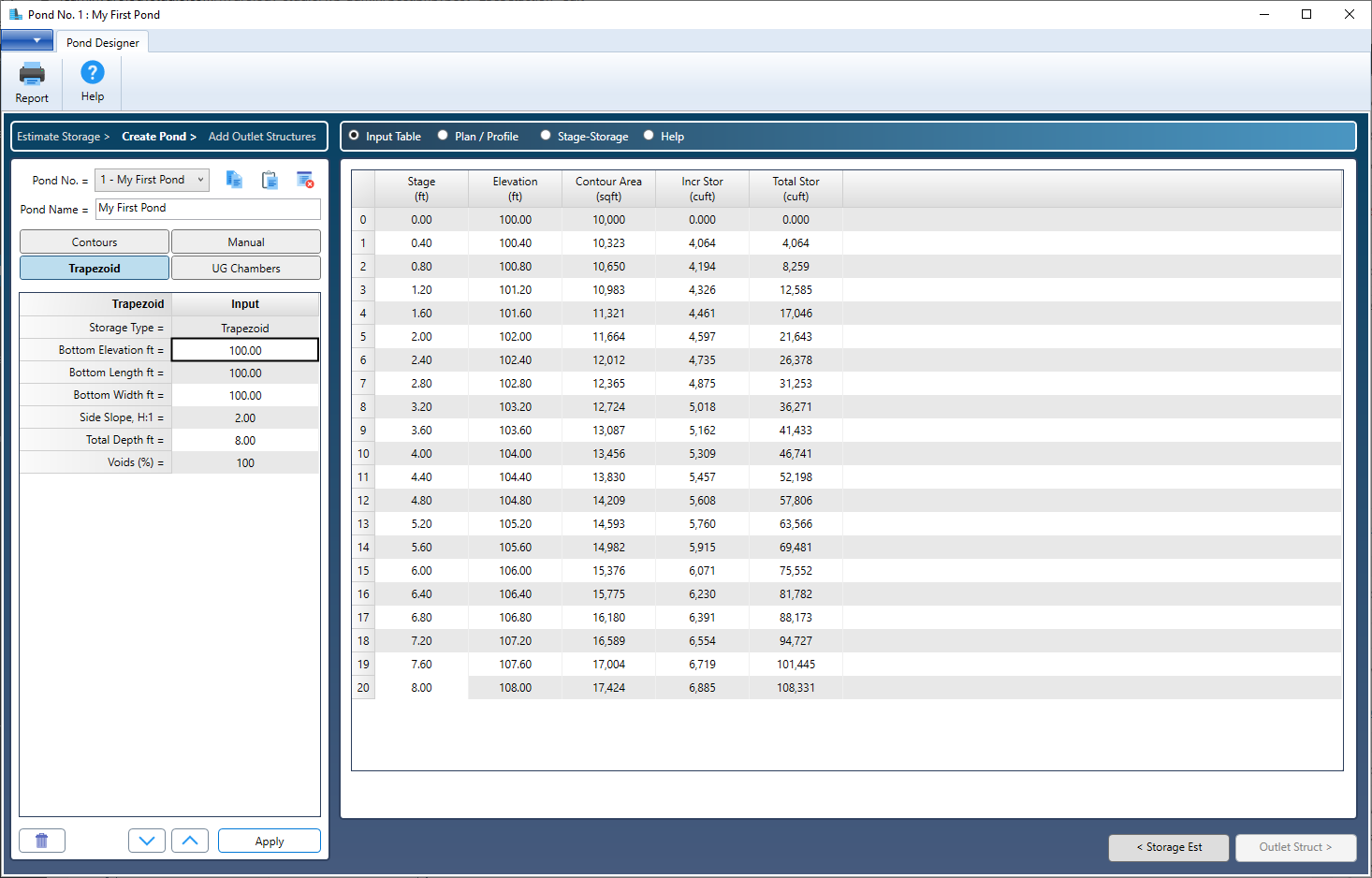
Click on the Help radio button on this screen to view input diagrams of each. For this tutorial we’ll opt for the Trapezoidal-shaped pond, just to keep things simple. Please select Trapezoid and enter the input parameters as shown below and then click [Apply].
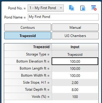
A pond with a bottom length and width of 100.00 feet and 2:1 side slopes has been selected. A total depth of 8 feet should provide us with one foot of free-board.
But that’s larger than the estimate! You’ll see on the output table that this configuration provides us with around 90,000 cubic feet at 7 feet of depth. Yes, it’s above the estimate by about 10 percent at 7 feet. Always make your pond slightly larger than the estimate to insure a successful initial routing. You can always return back to this step to make adjustments to your pond size.
Now click the [Outlet Struct] button on the lower right to move to the third and final step of our design, “Add Outlet Structures”.
Step 3 – Add Outlet Structures
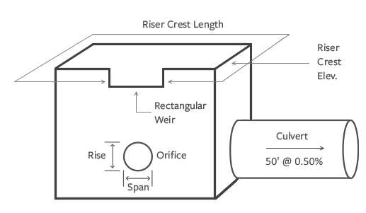
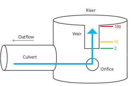
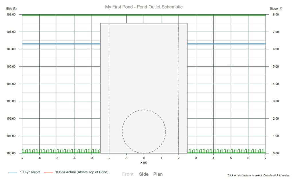
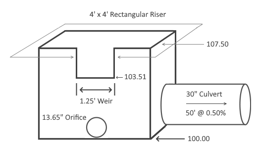
Now we will design the pond’s outlet devices using a multi-stage configuration in order to control three return periods… 2, 10 and 100-year. The structure will look like the one shown below that uses a Culvert and a Rectangular Riser to contain an Orifice and a Rectangular Weir. The Orifice controls the 2-year while the Rectangular Weir controls both the 10 and 100-year events. The Culvert’s sole purpose is to convey water out of the pond. Nothing else.
Hydrology Studio employs a powerful and clever feature that allows you to add outlet structures, one at a time, and perform intermediate trial routings along the way so that you experience a direct path to a final and elegant solution. It is highly recommended to add and design these outlet devices starting at the most downstream device and working in an upstream direction, not by increasing return periods.
Always Add the Culvert First
Lets begin by adding a 24-inch (a guess) diameter pipe resting at the pond bottom, 50 feet long at 0.50 percent slope. Click on the Culvert selector and add the data parameters as shown and click [Add/Update] to compute the Stage Discharge curve.
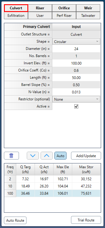
Next, perform a trial routing by clicking the [Trial Route] button and observing the results in the Trial Table at the bottom part of the input grid. Note that we are only interested in insuring the Culvert can pass the highest Target Qs, the 100-year event in this case, without restricting the flows.
The 100 year frequency row indicates that the Q Target is 36.46 cfs (from the Pre-developed hydrograph) and the actual routed peak Q is lower at 33.84 cfs. While this may satisfy our release rate requirement, it puts the Culvert in control which is not desirable.
Assuming a 27-inch is unavailable, change the Diameter to 30 inches. Then click [Add/Update] and [Trial Route] again.
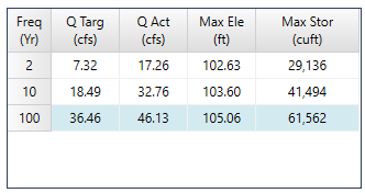
The Q Actual is now 46.13 cfs and is greater than the Q Target so we will accept the 30 inch.
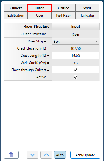
Add the Riser Structure
Before moving ahead with other outlets we must add a Riser structure, only to house the Orifice and Weir. To get a view of our structure, click on the Structure radio button at the top of the output table.

Add a 4 ft by 4 ft box-section Riser with a crest elevation at 107.50 to keep it well above the Max Elevations of the other routings. We do not want the Riser to control any flows or allow flow to enter over the top.
Click on the Riser selector and add the data parameters as shown below and then click [Add/Update]. Do not click the [Trial Route] button this time.
Add the Orifice (2-yr)
Still working upstream, add the Orifice, which controls the 2-year event. We need to add an orifice that only allows a Q Actual of less than or equal to the Target Q of 7.32 cfs.
An educated guess says a 12-inch diameter orifice will be a good starting point. Click on the Orifice selector, choose Orifice 1, and add the data parameters as shown below and then click [Add/Update] to compute the Stage Discharge curve.
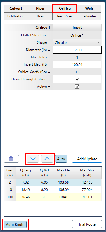
Next, perform a trial routing by clicking the [Trial Route] button and observing the results in the Trial Table.
Tip: Use the Interactive Tools – You can also place your cursor on the Diameter input and then click the [Up Arrow] button. If [Auto Route] is toggled ON you’ll get instant results with each arrow click. This will become your method of choice as you get more familiar with Hydrology Studio.
The 2-year row indicates the 12-inch produced a Q Actual less than Q Target. To minimize storage we should “dial this in” so that the Q Actual equals Q Target. This is easily done with Hydrology Studio by using the real-time interactive controls. Continue adjusting the Diameter with the [Up Arrow] until you’ve reached your goal.
So give that a try. You’ll find the answer at 13.65 inches. The Trial Route results will look like this. Pay no attention to the other frequencies for now, just the 2-year.
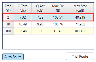
Perfect! The two Qs match exactly at 7.32 cfs.
Add the Secondary Weir (10 and 100 yr)
As they say, “Onward and Upstream”. Lets go upstream. This structure works “double-duty” in that it satisfies both 10- and 100-year criteria. Here we have to obey 18.49 cfs as well as 36.46 cfs Target Qs.
To add a Rectangular Weir click on the Weir selector, choose Weir 1, and add the data parameters as shown below. Note that the weir Crest Elevation is set to the Max Elevation computed from the 2-year event at 103.51. We’ll try a Crest Length of 1.00 ft to start.
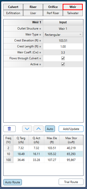
Then click [Add/Update] to compute a new Stage Discharge curve and if Auto Route is ON, you’ll see an updated routing table as well. If not, click [Trial Route].
The 10-yr row shows the Q Actual is below the Q Target. Same for the 100-year. This solution technically satisfies our requirements but we can improve this by adjusting the weir Crest Length to maximize the Q Actual, minimizing the storage required.
Just like you did with the Orifice, use the interactive tools. Click on the Crest Length input box. Then click on the [Up arrow] key until the Q Actual(s) are as close to their respective Q Target(s) as they can get without exceeding them. You should arrive at a result like this:
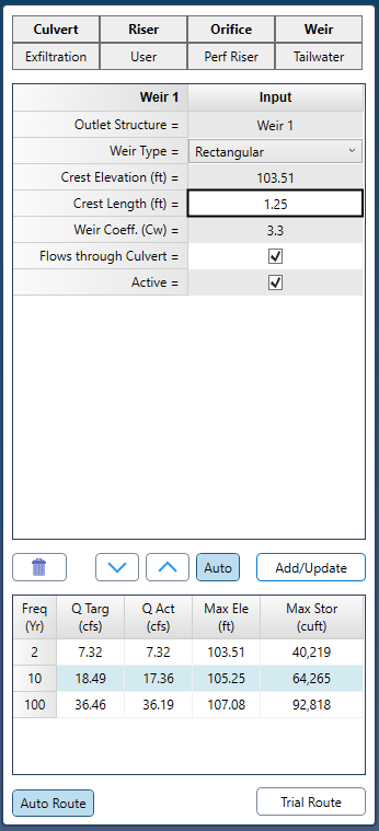
The best Crest Length is 1.25 feet wide. The 2-year, 10-year and 100-year criteria are now met. The Maximum Elevation came in at 107.08 providing us with nearly 1 foot of pond free-board. Notice that the design used 92,818 cubic feet of storage which is about 10% more than what was estimated.
Detention Pond Design Complete
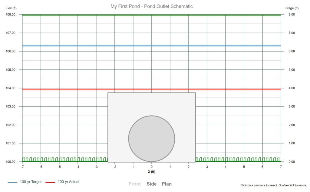
This pond design is now complete. Note that the Riser dimensions can be modified without having any effect on the hydraulic performance. For example, it can be a 5′ x 5′ Riser instead of 4′ x 4′. Just be sure its Crest stays above the 100-yr max. elevation.
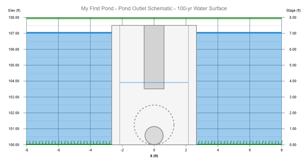
Click the rows on the Routing Table above to see the corresponding water surface. Use the Front Side & Plan links just beneath the drawing to view different sides of the structure.
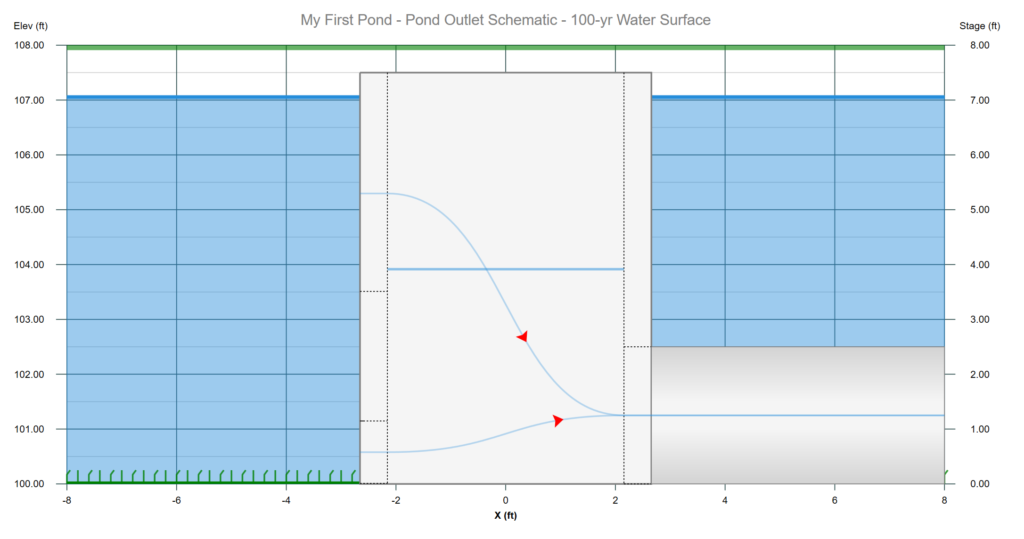
You may also be interested in viewing the Stage vs. Q curve, Trial Hydrographs, Drain Time, etc. available by the radio buttons above the Schematic.
Remember, all we have done up to this point is “design” the detention pond. We still need return to our Basin Model where we left off to complete the “real” routing.
Now click the [Finish] button at the lower right to return to the Basin Model where we will complete the project. You should see the following screen.
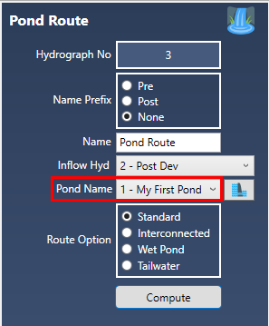
The Pond Name should now read “1 – My First Pond”. Next click [Compute] to perform the final routing. Then Click the Charts tab to view. Select all three hydrographs from the List on the left to overlay as shown below.
Print Reports
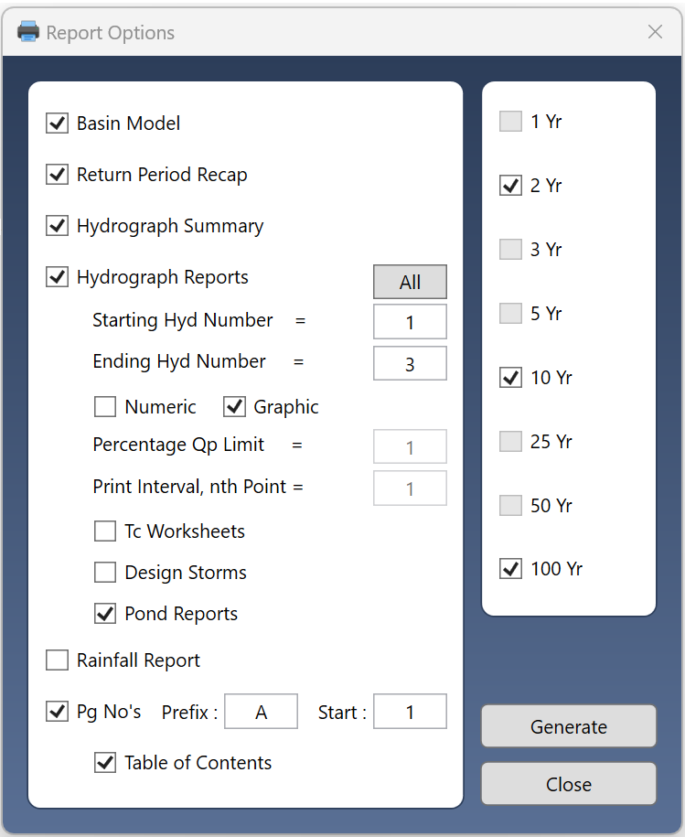
Click the [Reports] button on the top toolbar to print out final reports for submitting to approving authorities. You’ll have a lot to choose from. Be sure to include the Pond Report. These are commonly added to the Appendix of your formal drainage study.
Conclusion
You are now better equipped to proceed with your own real-life pre- and post-development detention pond designs. Just remember to follow the steps outlined above. Give your pond plenty of storage. Design outlet structures working from downstream to upstream, one device at a time. Try not to use the Culvert or Riser structure to control the outflows, rather use secondary devices that give you more precise control, and thus a more optimized and economical design.
If you find yourself struggling to get an outlet design to work, try increasing the size of the pond and then redesigning the outlet structure. Make sure the Culvert is not too small. Try different outlet device types, for example, the design above could have been done using a secondary Orifice rather than a Rectangular Weir.
You can download an actual project file that is very similar to this one here.