
How many times have you calculated the energy grade line for a storm sewer system… by hand? That’s what I thought. I’ve been in this business for over 30 years and can count on one hand the number of times I have. You can do it, but why? We have Desktop PCs on our desktops. But just in case you are of the “That’s what I thought” crowd or you’ve been depending on a spreadsheet for this, then please read this article. It’s goal is to:
- Educate you so that you know what you’re talking about, and reviewers know it.
- Educate the reviewer so the reviewees know that you know what you’re talking about.
- Empower you. Knowledge is power in the field of stormwater modeling.
When you’re done reading this you will be ahead of your peers with a stronger understanding of storm sewer hydraulics. You’ll be able to know if a storm sewer has been properly designed by just glancing at the hydraulic profiles.
We’re going to begin with a fluid mechanics review (sorry, it’s a prerequisite) and end with learning the proper way to calculate water surface profiles (HGL and EGL) for a storm sewer. Don’t worry, we aren’t going to do this by hand. But you will understand this as if you did it by hand. Let’s get started…
Three Things That Matter
I have this advice for anyone in civil engineering industry, especially those in site development or coming out of college with a BSCE. If you remember only three things from your Fluid Mechanics class, let it be these. Without them in your drainage design toolbox, you’ll be walking with a limp.
1. The Continuity Equation
Where:
Q = Flow (cfs)
V = Velocity (ft/s)
A = Cross-sectional area of flow (sqft)
This nifty little equation stands tall as it will never fail you. You will find it most handy when designing or analyzing storm sewers or open channels. In my early years in the software business a day rarely passed without a tech support call regarding the velocity in a storm sewer pipe. And of course my standard reply involved yet another introduction to the Continuity equation.
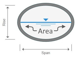
No matter what, velocity always, always equals the flow divided by cross-sectional area. Don’t depend on Manning’s equation for this. Put that away. If you’re looking for velocity look no further than the actual cross-sectional area in the pipe. Divide Q by that and viola… the correct velocity, guaranteed.
As you’ll learn below, the cross-sectional area is rarely what your Manning’s calculator wheel says it is. To know the Area is to know the hydraulic grade line (HGL). Keep reading…
2. The Energy Equation
It’s the granddaddy of all H&H equations. There’s so much you can do with the energy equation it’s mind boggling. To explain it in its entirety is beyond the scope of this lesson. But for now, let’s stick to H&H for civil engineers. Orifice equations, weir equations, Bernoulli equation, etc., all derive from the Energy equation.
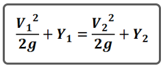
And that energy is made up of two parts, Potential and Kinetic. In our world, potential energy is Elevation Head (HGL) in feet (Y) and kinetic energy is V2/2g, a.k.a. Velocity Head. Nice and simple.
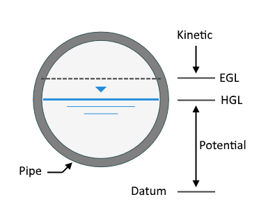
The total energy, we call EGL, is the sum of HGL and Velocity Head.
3. Manning’s Equation
I know, I just told you to put this thing away. You can get it back out now.
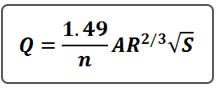
Every civil engineer has seen this equation a time or two and it doesn’t need much of an introduction, but it does need an explanation. Surprisingly, my 650-page fluid mechanics text book only dedicated a half-page to its description. It was named after someone who never stepped a foot in a fluid mechanics class, Irishman Robert Manning. He did not receive any education or formal training in fluid mechanics or engineering. He had an accounting background.
Manning’s equation is used primarily to determine energy loss due to friction implied by the n term, roughness coefficient. The A term is the actual cross-sectional area of flow. R is the hydraulic radius which is A divided by the wetted perimeter of that A. The equation is reliable up to about a 6 percent slope. That’s easy enough.
What puzzles many engineers is the S term. S is the slope. But it’s not the slope of the channel bed or pipe invert. Always remember this… It is the slope of the energy grade line (EGL). Period.
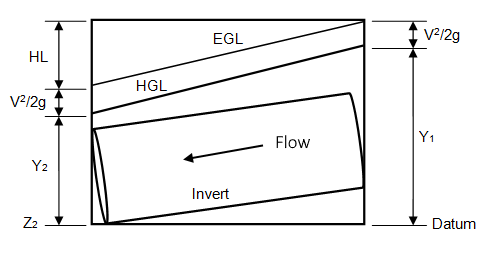
Choose any two points along a pipe or open channel for example. Add up the kinetic energy, and the potential energy, (Y) at each point. That sum is the total energy at that point or EGL. S is the slope of the line between those two points. The difference between the two EGLs represents the loss of energy due to friction, HL. It’s clever for storm sewer designers to set the pipe slope equal to S. That way the EGL runs parallel to the top of the pipe. Possible, but not always practical.
Understanding Full-Flow Capacity
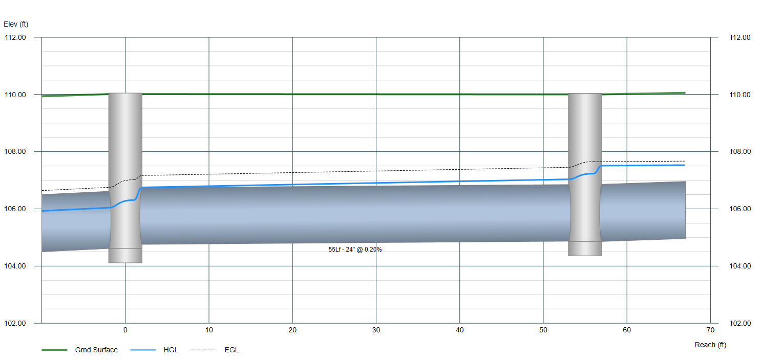
This is one of the most misunderstood terms in storm sewer hydraulics. So let’s set it straight. Full-flow capacity is simply the flow rate (Q) as computed by Manning’s equation, setting the slope, S, equal to the slope of the pipe invert and cross-sectional Area at full depth. That doesn’t mean the pipe cannot convey more than that, or less. It’s okay for pipes to pass a Q higher than the “full-flow capacity”. As shown in the illustration above, that pipe is carrying a flow that is higher. The tell-tale sign is the slope of the EGL being greater than the invert slope. Again, S in Manning’s equation is the slope of the EGL.
Calculating the Water Surface Profile
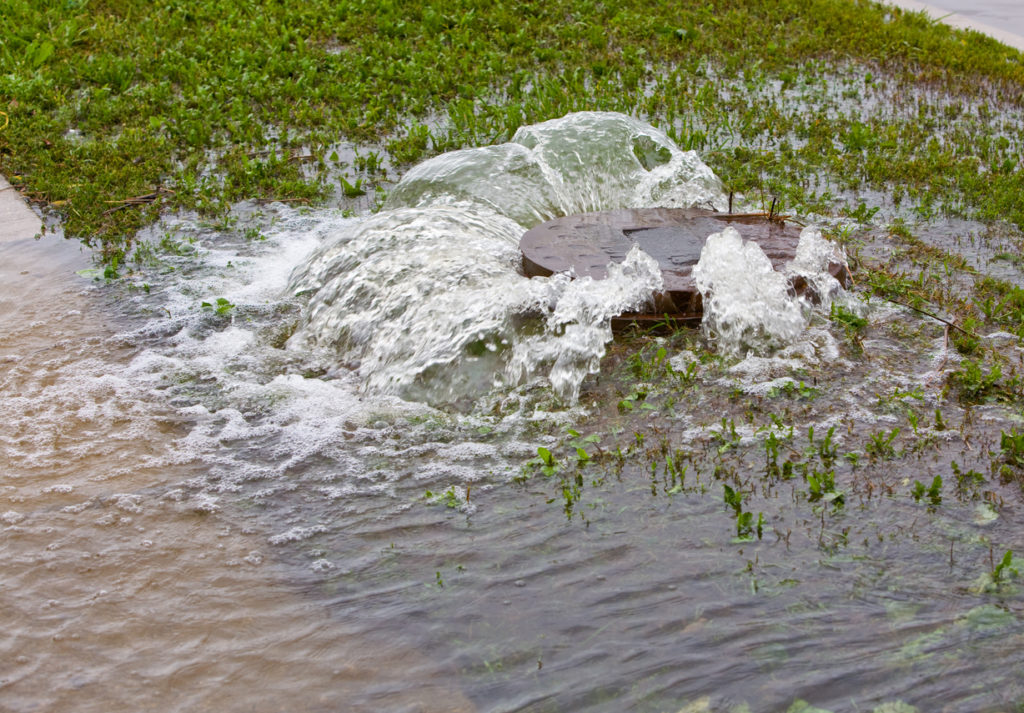
Now that we’ve passed basic fluid mechanics it’s time to put that knowledge to work on computing water surface profiles in a typical storm sewer. We need to know if our systems are blowing off manhole covers or breaching inlets, right?
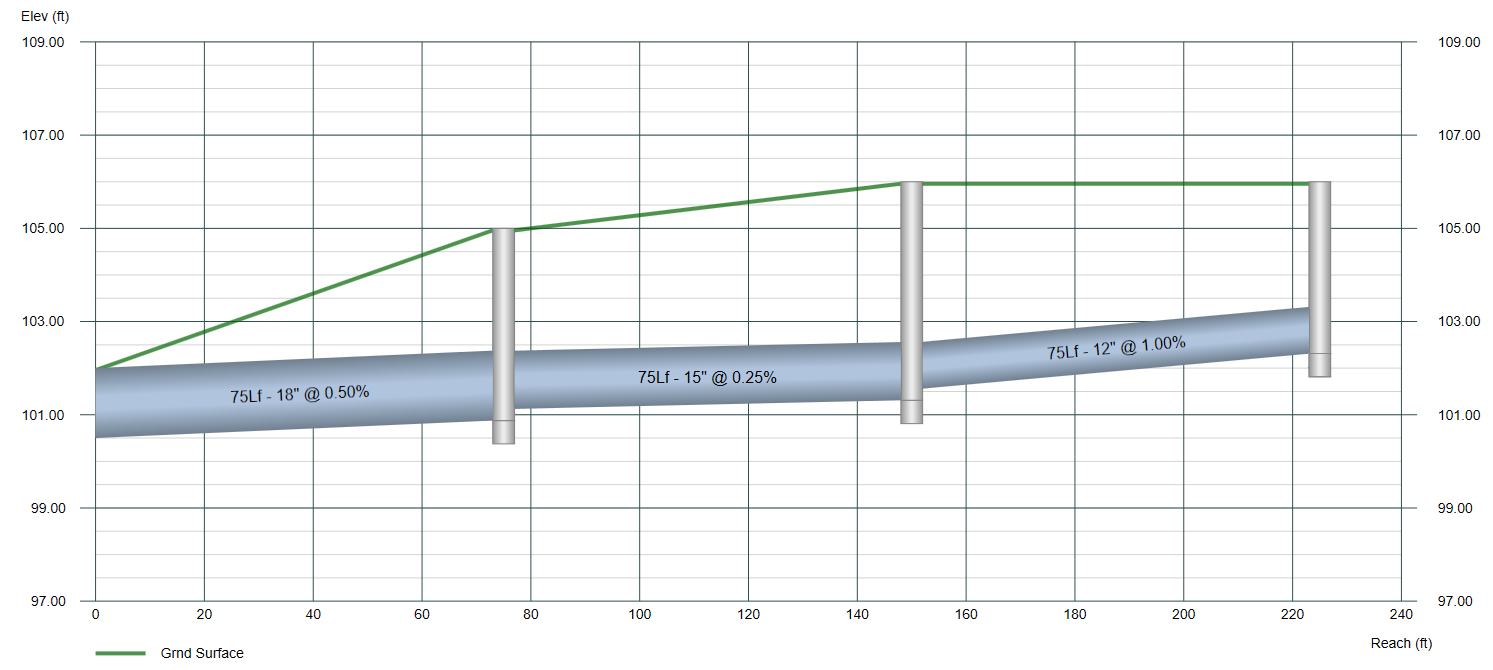
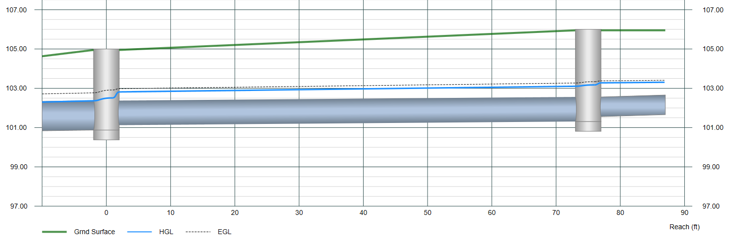
Below is a profile of an existing three-line storm sewer. It has already been designed, flow rates established, etc. but needs a water surface profile for a higher storm event. We will use what’s known as the Standard Step method.
In essence, the process involves 4 steps, in this order, beginning at the downstream end and working upstream, Line-by-Line. (A “Line” is a length of pipe with a junction at its upstream end.)
- Set the starting energy elevation (EGL Dn).
- Calculate the energy profile for the pipe (EGL Up).
- Calculate the Head Loss at the upstream junction.
- Add the Head Loss from Step 3 to the EGL Up from Step 2. (This becomes the beginning energy (EGL Dn) for the next, upstream Line.)
Repeat Steps 1-4 for each Line until you’ve reached the end. Sounds pretty simple. Lets go through these steps one-by-one.
Step 1 – Set the Starting EGL
For the beginning Line this step is quite simple. Most of the time a downstream water surface, HGL, is known, commonly called a tailwater (Tw). The Starting EGL is simply the HGL + Velocity Head (V2/2g). This is where you break out your Continuity equation, Q = VA, and calculate V based on the cross-sectional area, A, of the flow in the pipe.
If Tw is unknown, it is safe to assume one of the following:
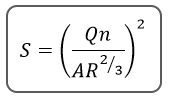
- Normal Depth – This is a depth defined by Manning’s equation where S and the slope of the invert are assumed equal. Manning’s equation can be arranged into the form: Qn / 1.49S1/2 = AR2/3 where the left hand side of the equation is a constant that can be calculated from the specified values for Q, n, and S. On steep slopes, Normal depth can be less than Critical depth. In these cases use Critical depth instead.
- Critical Depth – This depth is where the Energy (EGL) for your particular Q is at a minimum. In other words, for all of the possible combinations of depth and it’s resulting velocity head, this one represents the smallest EGL. Water does not prefer to be at this depth as it is unstable and will tend to quickly shift into higher or lower depths. For this reason, Critical depth as a starting Tw is not your best choice.
- Full Depth – Assume the depth is at the top or crown of the pipe. Always a safe and conservative choice.
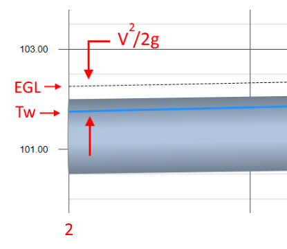
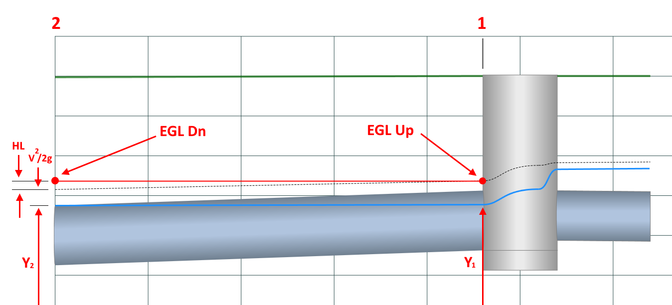
The above shows the starting EGL at the Outfall based on a known Tw elevation. It’s not as easy to determine for the remaining pipes. We’ll revisit this step later…at the end of Step 3.
Step 2 – Calculate the EGL for the Pipe
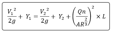
This is where we use the Energy Equation but with a twist. We’re going to add Head Loss (HL). That is, the energy loss due to the pipe’s wall friction. Because of this, we use a unique form of the energy equation derived from Bernoulli that includes Manning’s equation.
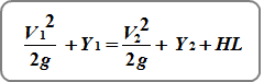
Where all of the terms on the left side of the equals sign refer to the upstream end (EGL Up) and those on the right refer to the downstream end (EGL Dn). HL is given to us by Manning as Slope of the EGL (S) x Pipe Length (L) where:
We already know the EGL Dn from Step 1. The goal now is to find the EGL Up using our new energy equation. Here it is in its full form with S x L in place of HL.
Where:
n = Manning’s n roughness coefficient
A = cross-sectional area of flow
R = hydraulic radius
L = pipe length
Q = flow rate
g = gravity
V = velocity
A solution to this equation requires an iterative-based procedure. We only know V and Y at Point 2 (downstream). So we have to assume a Y at the upstream end, Point 1. Then compute A, V and V^2/2g. From that comes the EGL Up. Compare to EGL Dn + HL. If they don’t match within a desired tolerance, like 0.01 feet, the assumption was incorrect. Repeat with a new assumed Y.
When the flow depths are less than full, use an average S (slope of the EGL) by computing it for both upstream and downstream ends and averaging it, Sa = (S1 + S2)/2.
Your key takeaway here is that it’s all about the EGL, not HGL, and to know that the proper water surface profile in a pipe requires a solution to the Bernoulli Energy equation.
There must be a balance in energy between the two ends of the pipe. The EGL at Point 1 must equal the EGL at point 2 plus HL from Manning’s equation. If the slope of the EGL is greater than the invert slope, it tells you that the Q is greater than the “Full-flow Capacity”. If the slope of the EGL is less, then you’ll know the Q is below capacity. In the latter case, you should consider decreasing the pipe size if this is a new design.
Step 3 – Calculate the Junction Loss
Calculating the head loss at the upstream junction can be more difficult than computing the loss in the pipe. Modern-day analysis expects the consideration of multiple components of flows inside of a structure. These are describe in detail in HEC-22 and AASHTO and are outside the scope of this article. These losses are typically a function of velocity. Those include computing, step-by-step, in the upstream direction:
1. Entrance Loss – Determines an initial energy level based on either inlet control (weir and orifice) or outlet control (partial and full flow) equations.
2. Additional Losses – Makes adjustments to the Entrance Loss and are based on benching (shape of the bottom of the structure), angles of incoming lines, and plunging flows (flows dropping from inlets and incoming pipes that are above the crown of the outgoing pipe).
These adjustments can be positive or negative. For example, benching tends to reduce energy losses in which case you may see the EGL line decrease across the junction. In all cases, the adjusted energy level cannot be below the initial energy level as computed in Step 1. Sorry!
3. Exit Loss – An exit loss is computed from each inflow pipe and is added to the adjusted EGL in Step 2. This newly computed energy level is used as the starting energy (EGL) for the incoming line(s).
Rather than hand-calculating the losses here it’s more important to introduce what goes into determining the losses at junctions. Remember, these losses are “Energy” losses, not direct changes in the water surface (HGL).
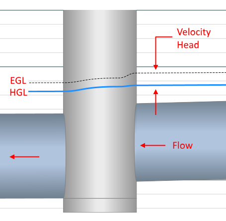
As you observe in the junction above, there’s an increase in the EGL across the structure as you move upstream. In fact there’s two. The first bump you encounter comes from the Entrance Loss and Additional Losses (adjustments). The second bump up is the Exit Loss which finally brings you to the EGL at the upstream end of the junction.
Step 4 – Setting the EGL Dn for the Incoming Line
The EGL you just computed becomes the starting EGL for the incoming Lines. All of them will use this one EGL. It is from this EGL that the incoming pipe’s HGL is determined. NOT the other way around! You may stumble across some online literature that describes otherwise. Don’t fall for it. Because if you do, that’s what you’ll likely see, a fall in the EGL going upstream. A negative energy loss is sure to raise the eyebrows of a critical reviewer.
The HGL is a component of the EGL. Remember that total energy equals the potential head plus the kinetic head at any given point. The HGL is the EGL minus the Velocity Head.
Returning to the picture above you notice the EGL takes a slightly different path upstream than the HGL. By glancing at this you can easily determine that the upstream pipe has a higher velocity than the outgoing pipe. It’s true because it has a smaller cross-sectional area. The incoming pipe is a 15-inch. The outgoing is an 18-inch.
Summary
So there you have it. The basic skill and knowledge of how to calculate a water surface profile for a storm sewer. It’s simply repeating a 4-step process which begins at the downstream end of your system working towards the upstream end. The Bernoulli Energy equation is used to compute the EGL within the pipe and a separate procedure is used to calculate the junction losses.
The entire process is governed by the Energy Grade Line (EGL) not the water surface. The water surface (HGL) is a byproduct of the EGL, i.e., EGL minus the velocity head.
When the Energy Equation Fails
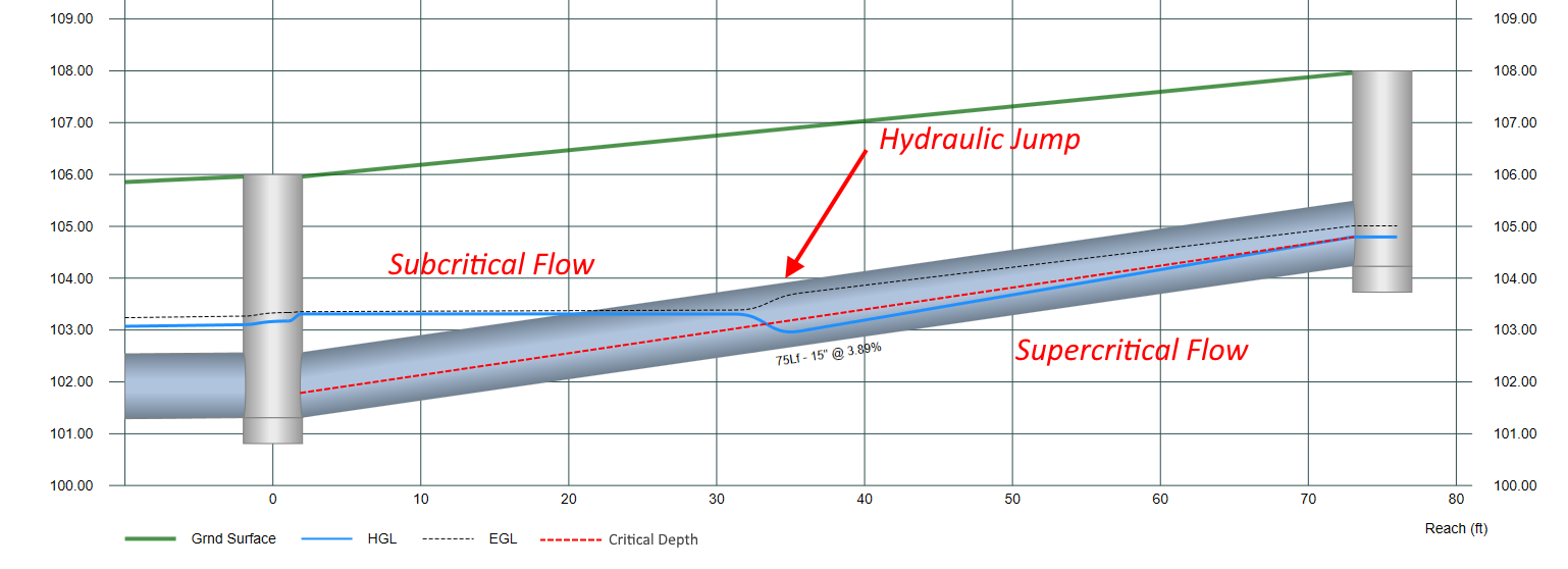
There are exceptions or special cases where the above procedure for computing the EGL in the pipe fails. There will be times when the energy equation cannot balance no matter how many trials or iterations you execute. This occurs with steeply sloped pipes and the downstream depth is subcritical and actual flow depth upstream is supercritical as shown below. In other words, HL is so large that Manning’s Equation cannot account for it all.
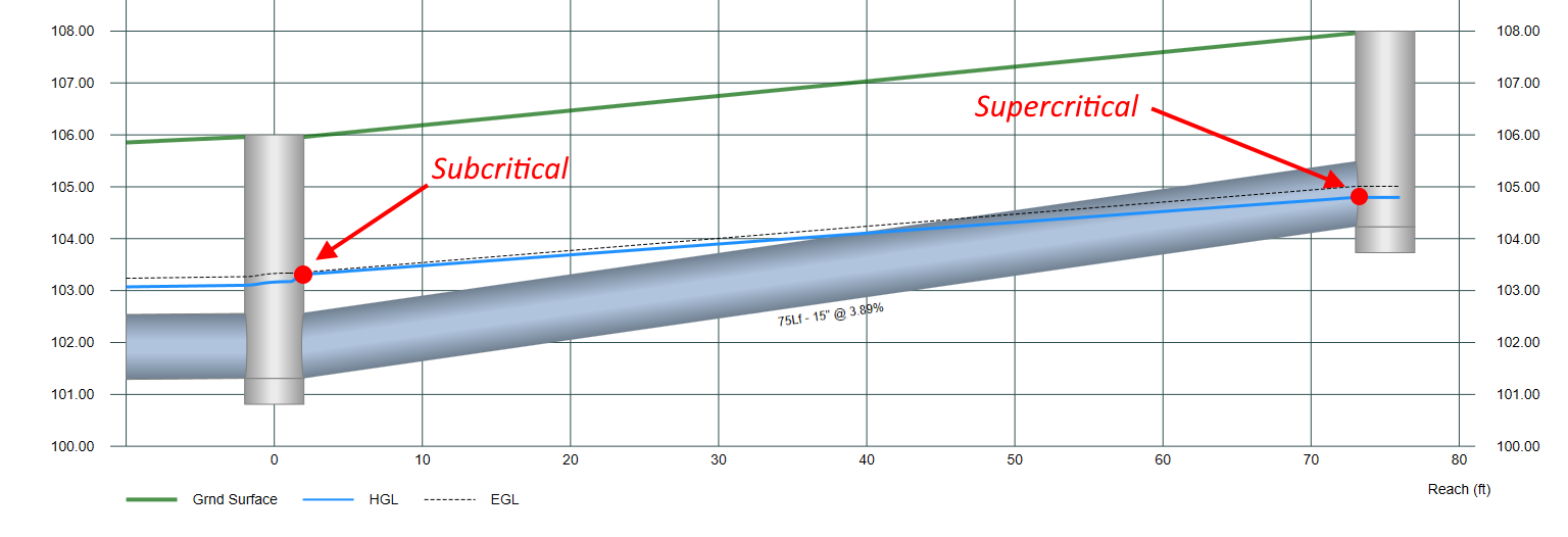
The HGL in this case could not be found by our traditional solution so we must assume Critical depth upstream and resume our normal procedure. (Note that per HEC-22, junction losses are ignored when critical depth occurs.)
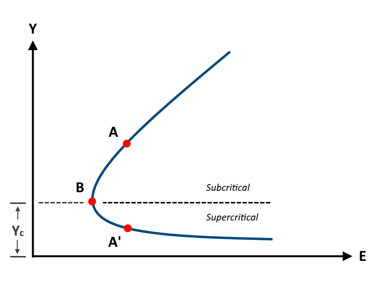
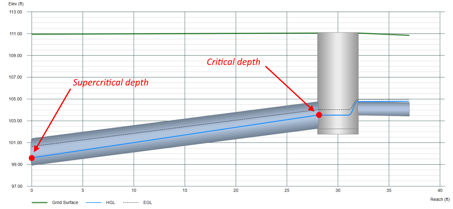
To explain, consider this Energy vs. Y curve where Y is the depth of flow in the pipe and Yc is Critical depth. E represents our EGL. Point A is our downstream depth and Point A’ is the depth upstream where we are trying to get to as in the example profile above.
Our flow depth must follow along the E vs. Y curve. We can’t jump across the space which separates A and A’. We must pass through Point B. But whenever the water surface passes through Critical depth, the energy equation is not applicable. It is only applicable to gradually varied flow situations and this is a rapidly varied flow condition. So we can only calculate the EGL on the top side of Critical depth, or the bottom. But not both at the same time. They must be performed separately.
To solve this problem we assume Critical depth at the upstream end. This takes care of the Subcritical profile above Yc. Next we perform the exact procedure as in Step 2, but reversed. Calculations progress from the upstream towards the downstream because our known Tw is now at the upstream end, Critical depth. This profile stays below the Yc line and is termed the Supercritical profile.
Staying on either side of Yc keeps us from violating the “gradually varied” flow rule. But now we have two profiles! Which one is correct?
We do indeed have a conflict between the upstream and downstream controls, both of which influence the same pipe.
The upstream control causes supercritical flow while the downstream control dictates subcritical flow. This conflict can only be resolved if there is some means for the flow to pass from one regime to the other.
Introducing the Hydraulic Jump
As you learned so far, Manning’s equation can account for energy losses due to pipe friction, thus the n value. But it cannot account for losses that occur when transitioning between flow regimes. Experimental evidence shows that there is a way to get through this transition via a phenomenon known as a hydraulic jump. Think of hydraulic jumps being synonymous with sonic booms, when jet aircraft break the sound barrier. A process often accompanied by extreme turbulence and high energy losses. Once we pass through this, things get back to normal.
The challenge is how to model this large energy loss. Since Manning’s equation has left the scene, we’ll need to use some other concept of piecing together these two profiles… Momentum.
Downstream vs. Upstream
The Momentum Principle is ideal for determining depths and locations of hydraulic jumps. Think of this as a contest between the upstream guys and the downstream guys. Each team attempting to push the other out of the pipe. The contest usually ends up a tie, somewhere in the middle.
The procedure computes momentum (M) at certain points along the pipe, say every 5 feet. One for the subcritical profile (M1), and one for the supercritical profile (M2). Both at the same reach locations. As we move along downstream in the pipe, these momentums are compared to each other. When M1 > = M2, it is established that a hydraulic jump must occur at this point.
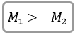
Momentum, M1, of the subcritical profile must be greater than or equal to the momentum, M2, of the supercritical profile.
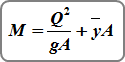
Where:
Q = Flow rate
A = Cross-sectional area of flow
Y = Vertical distance from the water surface to the centroid of A
The location of the jump is somewhere along the pipe’s length when M1 = M2.
If M2 continues to exceed M1, then the upstream force is stronger than the downstream force and the jump just gets pushed all the way through the pipe.
No hydraulic jump. The upstream guys win.
Learn more about Hydrology Studio’s complete suite of stormwater design software.
- Hydrology Studio
- Stormwater Studio
- Culvert Studio
- Channel Studio
- Studio Express
Visit Hydrology Studio today.