
In the realm of modeling open channels, having a deep understanding is crucial for ensuring job stability. As previously stated, my goal is for you to stand out as the most knowledgeable individual in the conference room when discussions on hydrology and hydraulics arise. This piece intends to further enhance your expertise in the field of hydrology and hydraulics.
In almost every site development project there’s an open channel around the corner that needs to be dealt with. Just the mention of “backwater curves” or “floodplain encroachment” intimidates project stakeholders. Like deer in headlights, they instinctively freeze. Some brave sole breaks out the acronyms, HEC-2, HEC-RAS, HEC-[insert suffix here], WSPRO, FEMA, and more acronym-based software. Suddenly the project gets complicated and the conference room gets quiet.
Just the mention of “backwater curves” or “floodplain encroachment” intimidates project stakeholders. Like deer in headlights, they instinctively freeze.
Hands up from all those people who have hand-calculated a water surface profile for an open channel. Anyone?
Fear no more. Open channel hydraulics is not as difficult as its reputation has made it out to be. There are two reasons why many civil engineers fear open channel hydraulics:
- They realize they didn’t get sufficient training in college.
- The industry has been influenced by governing authorities, leading to the creation of misperceptions and a certain stigma. These misperceptions suggest that only computer programs issued by the government hold the capability to unravel complex mysteries, almost like a hidden code similar to that of Area 51.
This article aims to close the divide between academia and practical experience by equipping you with the necessary knowledge to tackle various subjects independently, free from government intervention. Additionally, you will develop the skills to efficiently grasp any open channel modeling software due to a deeper comprehension of the inputs and their functions.
It’s Easier Than You Think
Yes, calculating water surface profiles for open channels is easier than most engineers think. It’s easier than storm sewer systems, where you’re having to deal with those pesky junction losses, and it’s easier than modeling culverts with all those inlet control, outlet control, submergence concepts. With open channels there are no junctions, no inlets, no inlet control, none of that. There will be a bridge crossing from time-to-time which is discussed in Part III of this series… when completed. But even those procedures are easy work once you understand the basic concepts.
In just a few minutes, you will have a greater understanding of the basic calculation procedure which is the underlying foundation for successful open channel modeling. So here we go…
Three Things You Must Know
I have this advice for anyone in the civil engineering industry, especially those in site development or coming out of college with a BSCE and/or those of you with CFM attached to your title. If you remember only three things from your Fluid Mechanics class, let it be these. Without them in your drainage design toolbox, you’ll be walking with a limp.
1. The Continuity Equation
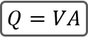
Where:
Q = Flow (cfs)
V = Velocity (ft/s)
A = Cross-sectional area of flow (sqft)
This two-term equation will never fail you.
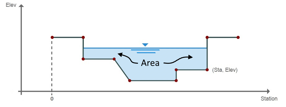
No matter what, velocity always, always equals the flow divided by cross-sectional area. Don’t depend on Manning’s equation for this. If you’re looking for velocity, look no further than the actual cross-sectional area of the water in the channel. Divide Q by that area and you’ll always get the correct velocity, guaranteed. What you should be looking for is the water surface, the hydraulic grade Line (HGL), that produced this Area. And to know the Area is to know the Energy Grade Line (EGL).
2. The Energy Equation
It’s the granddaddy of all H&H equations. There’s so much you can do with the energy equation it’s mind boggling. But for now, let’s stick to H&H for civil engineers. Orifice equations, weir equations, Bernoulli equation, etc., all derive from this Energy equation.
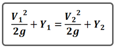
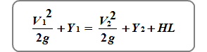
And that energy, at any given open channel cross-section, is made up of two parts, Potential and Kinetic. In our world, potential energy is Elevation Head (HGL) in feet (Y) and kinetic energy is V2/2g, a.k.a. Velocity Head. So at any point along an open channel, the energy is:
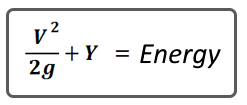
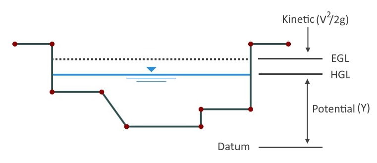
The total energy, EGL, is the sum of HGL and Velocity Head. What’s really cool is that the energy at one cross-section equals the energy at another cross-section, and another, and another. Knowing this, we can predict the water surface elevation pretty-much anywhere.
But there’s another visitor at this energy party, known as “Head loss” or HL for short. It’s actually not a loss, it just looks that way. It’s real energy that gets transformed into heat resulting from the friction between the water and the channel boundary, commonly called skin-friction drag. To quantify this loss we employ a special equation and insert it into our energy equation.
3. Manning’s Equation
Every civil engineer has seen this equation a time or two and it doesn’t need much of an introduction, but it does need an explanation.
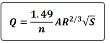
Manning’s equation is used primarily to determine energy loss due to friction implied by the n term, roughness coefficient. The A term is the actual cross-sectional area of flow. R is the hydraulic radius which is A divided by the wetted perimeter of that A. The equation is reliable up to about a 6 percent slope.
S is the slope. But it’s not the slope of the channel bed. Always remember this… It is the slope of the energy grade line (EGL).
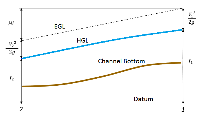
Choose any two points along an open channel, for example. Add up the kinetic energy, V2/2g, and the potential energy, (Y) at each point. That sum is the total energy or EGL. S is the slope of the line between those two points. The difference between the two EGLs represents the loss of energy due to friction, HL, and is S x distance between these two points (L).
Calculate the Water Surface
Now that we’ve passed basic fluid mechanics it’s time to put that knowledge to work on computing a water surface profile for an open channel. We’re simply going to combine the Energy Equation with Manning’s equation. Then it’s just a matter of solving that equation between two adjacent channel sections.
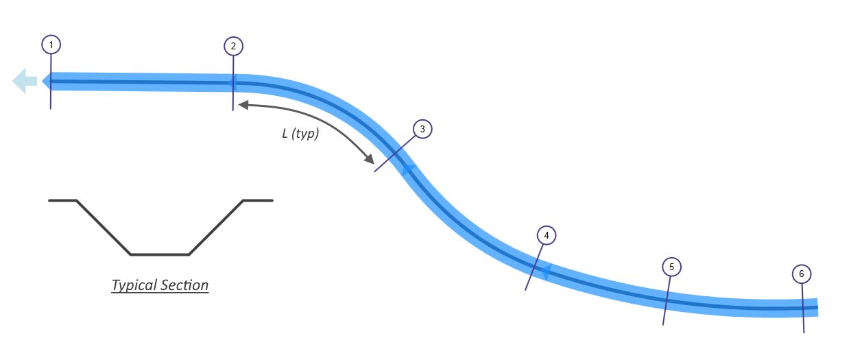
Below is a plan view of an open channel reach that contains six channel cross-sections. The channel sections are simple trapezoidal shapes at differing elevations and bottom widths. Flow rates have been established. All it needs is a water surface profile. We will use what’s known as the Standard Step method.
In essence, the process involves just 2 steps, in this order, beginning at the downstream end, Section 1, and working upstream, section-to-section, until we reach Section 6.
- Setting the beginning water surface elevation for the downstream section.
- Calculating the water surface elevation for the next upstream section. This becomes the beginning water surface elevation for the next, upstream section.
Repeat for each Section until you’ve reached the end. Sounds pretty simple. Lets go through these two steps one-by-one.
Step 1. Set the Starting HGL
For the very first section, downstream, you’ll have three choices:
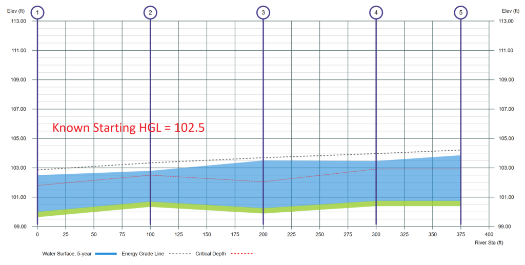
- Known Elevation – For the beginning Section, a water surface, HGL, is known, commonly called a tailwater (Tw). For the profile above, 102.5 was used.
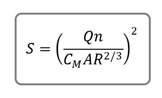
- Normal Depth – Use this when you don’t have a Known Elevation. This is a depth defined by Manning’s equation where S and the slope of the channel invert are assumed equal. Manning’s equation can be arranged into the form: Qn / 1.49S1/2 = AR2/3 where the left hand side of the equation is a constant that can be calculated from the specified values for Q, n, and S. On steep slopes, Normal depth can be less than Critical depth. In these cases use Critical depth instead.
- Critical Depth – This depth is where the Energy (EGL) for your particular Q is at a minimum. In other words, for all of the possible combinations of depth and it’s resulting velocity head, this one represents the smallest EGL. Water does not prefer to be at this depth as it is unstable and will tend to quickly shift into higher or lower depths. For this reason, Critical depth as a starting Tw is not always your best choice.
For all other sections, just use the HGL calculated from the previous section.
Step 2. Calculate the HGL for the Upstream Channel Section
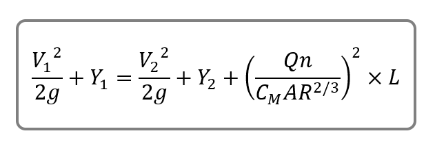
This is where we use the Energy Equation with the added Head Loss (HL) component.
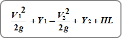
All of the terms on the left side refer to the upstream Section (EGL Up) and those on the right refer to the downstream Section (EGL Dn). HL is given to us by Manning rearranged as S x Reach Length (L) where:
CM = Manning Coefficient, 1.49 (1.00)
We already know the EGL Dn from Step 1. The goal now is to find the EGL Up using our new energy equation. Here it is in it’s completed form with S x L in place of HL.
Where:
n = Manning’s n roughness coefficient
A = cross-sectional area of flow
R = hydraulic radius
L = channel reach length (distance between the two Sections)
Q = flow rate
g = gravity
V = velocity
CM = Manning Coefficient, 1.49 (1.00)
A solution to this equation requires an iterative-based procedure. We only know V and Y at Point 2 (downstream). So we have to assume a water surface elevation, Y, at the upstream end, Point 1. Then compute Area, Velocity and Velocity Head. From that comes the EGL Up. Compare to EGL Dn + HL. If they don’t match within a desired tolerance, the assumption was incorrect. Repeat with a new assumed Y.
Once you have achieved an answer, repeat this process with the next upstream section and so on. The newly computed HGL is used for the variables on the left side of the equation.
In the real world, programs like Channel Studio, HEC-RAS, etc. will use an average S in order to better estimate the friction losses between sections. Known as the Average Friction Slope method.
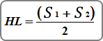
S1 refers to the upstream section, S2 refers to the downstream section.
Below are sample calculations from Section 1(downstream) to 2 (upstream) shown above.
The two channel sections are trapezoidal with 1:1 side slopes and 10-foot bottom widths. Manning’s n = 0.025. The inverts are 100.00 at Sec 1 and 101.70 at Sec 2. L = 100 ft.
We want to calculate the water surface at Section 2. We set the starting HGL at a known elevation of 102.50. From there we can calculate the parameters for the downstream side of the energy equation. Next we must assume an upstream Y. The first assumed Y is made by adding the depth of the downstream section to the invert of the upstream section, so (102.5 – 100.00) + 100.70 = 103.20. Educated guess, that’s all.
It is now a question of calculating the figures until the final discrepancy in the rightmost column is less than our accepted margin of 0.015 feet. The interesting part is that the outcome provides a hint towards resolving the issue. By taking half of the error and adding it algebraically to the previously assumed Y value, a solution can be promptly obtained. For instance, during the second attempt, Y = 103.00 was determined by 103.20 + -0.399 / 2. (-0.399 represented the error computed in the initial attempt).
| DOWNSTREAM | UPSTREAM | Error | |||||||||||
|---|---|---|---|---|---|---|---|---|---|---|---|---|---|
| Q | L | Y | Area | Vel | Vel Hd | E2 | Y | Area | Vel | Vel Hd | E1 | HL | E2 + HL - E1 |
| 150 | 100 | 102.50 | 31.25 | 4.80 | 0.358 | 102.86 | 103.20 | 31.25 | 4.8 | 0.358 | 103.55 | 0.291 | -0.399 |
| 103.00 | 28.23 | 5.31 | 0.439 | 103.43 | 0.341 | -0.229 | |||||||
| 102.88 | 26.52 | 5.65 | 0.497 | 103.38 | 0.379 | -0.141 | |||||||
| 102.80 | 25.54 | 5.87 | 0.536 | 103.34 | 0.406 | -0.074 | |||||||
| 102.77 | 24.96 | 6.00 | 0.561 | 103.33 | 0.424 | -0.046 | |||||||
| 102.75 | 24.63 | 6.09 | 0.576 | 103.32 | 0.435 | -0.025 | |||||||
| 102.73 | 24.43 | 6.14 | 0.585 | 103.32 | 0.442 | -0.018 | |||||||
| 102.72 | 24.32 | 6.17 | 0.591 | 103.31 | 0.446 | -0.004 | |||||||
| 150 | 100 | 102.72 | ... | ... | ... | ... | |||||||
| Units in feet | |||||||||||||
Interpreting Results
So that’s the basic calculation process. Applied to the sample six-section plan above reveals these profile results:
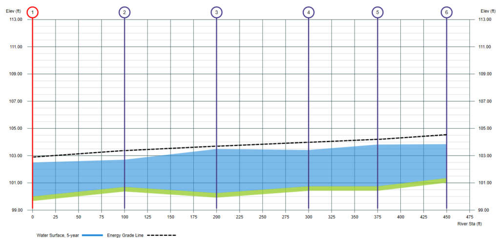
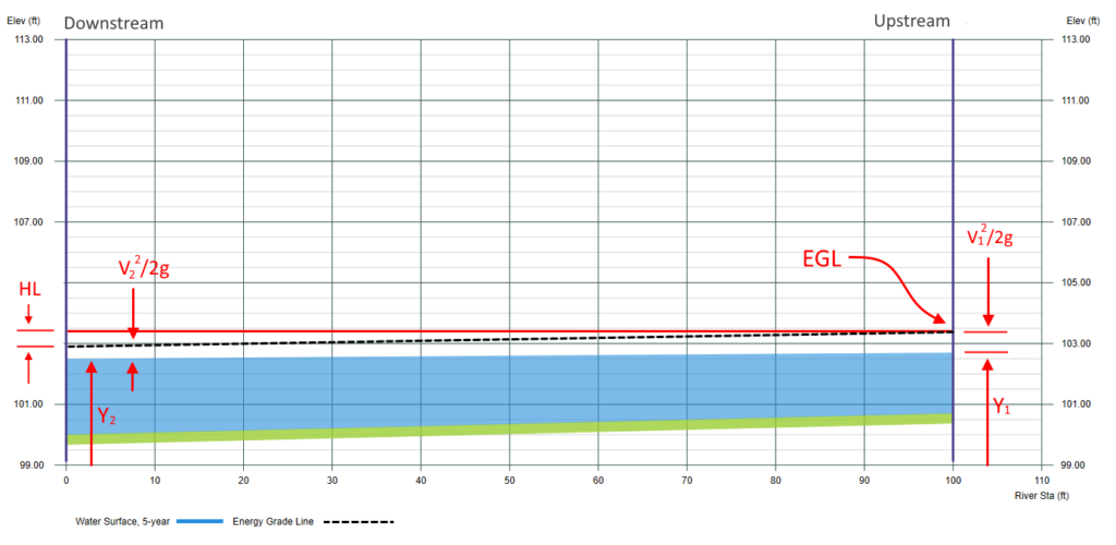
The inexperienced modeler may find themselves easily confused in this scenario. It is important to observe that the EGL (black dotted line) decreases as you progress downstream, which is expected as energy cannot be gained or created. However, it is crucial to note the fluctuation of the water surface between different sections. While the slope of the channel bed from Section 2 to 3 is adverse, the water surface remains unaffected. The water surface between Sections 3 and 4 slopes adversely due to the reduction in channel width from 10 to 7 feet at Section 4, leading to an increase in velocity and velocity head. Remember, the water surface is always equal to the EGL minus the velocity head, in this case, a resulting in a reduction in water depth.
Below is another interesting example of a simple trapezoidal-shaped channel with obstructions, similar to bridge abutments. Notice how they squeeze and reduce the area of the cross-sections. One would intuitively think that the water surface would rise as it flows through these abutments.
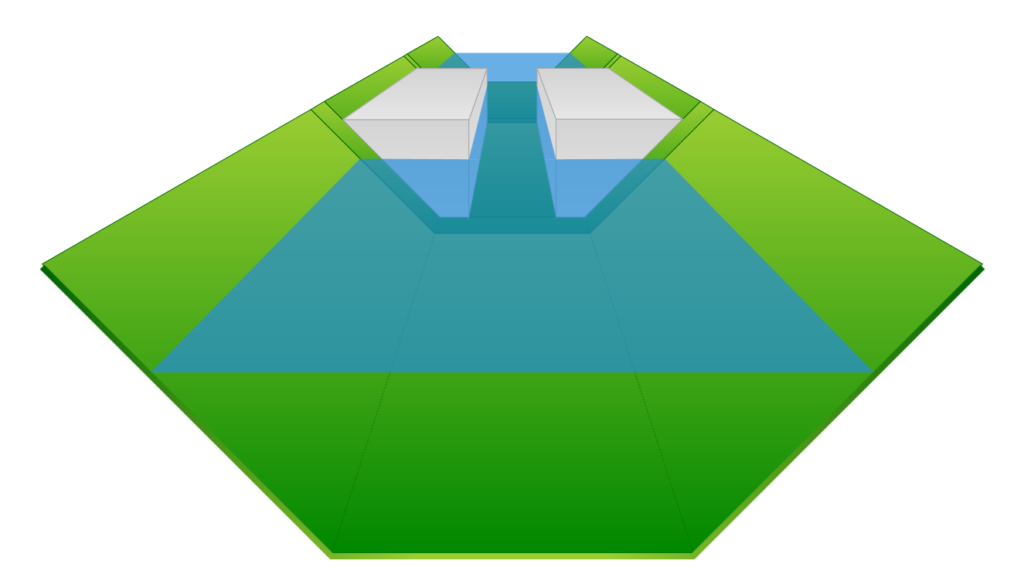
But in fact, it does just the opposite. The water surface drops!
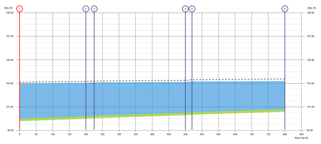
Remember the Continuity equation, Q = V x A ? The abutments indeed reduced A, so V must increase to maintain Q. Subtracting the increased velocity head (V^2/2g) from the black dotted line reveals the true water surface as shown in the channel’s profile below.
Things get back to normal downstream once the cross-sectional area enlarges and velocity slows, velocity head shrinks, HGL goes up.
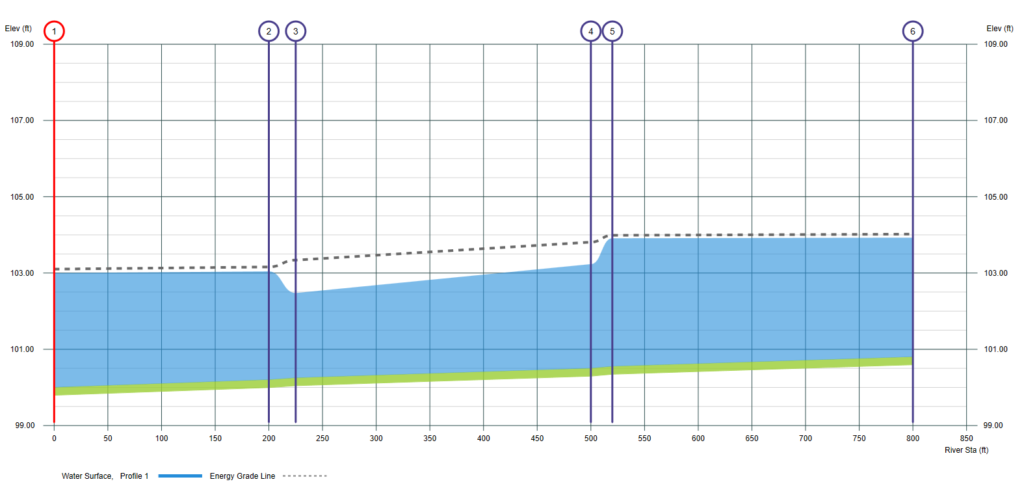
What’s interesting is that the water surface did rise. Over 0.50 feet. But not between the abutments. But rather at the sections just upstream, where the cross-sectional area was untouched. How’d that happen?
Remember Manning’s equation?
Between the obstructions we have a decrease in Area, A, and thus R. So slope, S must increase to maintain Q. Sure enough, the slope of black dotted line between sections 2 and 5 increased. It raised the EGL upstream at sections 5 and 6 where you have a full cross-section, lower velocity, higher HGL.
Always remember… anywhere along that black dotted line, there can be only one legitimate combination of water surface elevation and velocity head. Energy rules and the Energy equation will always provide an accurate answer, regardless of the channel’s shape or slope.
Summary
So there you have it. The basic skill and knowledge of how to calculate a water surface profile for an open channel. It’s simply repeating a 2-step process which begins at the downstream end of your system working towards the upstream end. The Bernoulli Energy equation is used to compute the EGL. The water surface (HGL) is a consequence of the EGL, i.e., EGL minus Velocity Head.
The aim of this lesson was more about understanding the mechanics of water surface profiles than actually crunching numbers. You’ll most likely use a computer for that, and you should. But at least now you’ll know what goes on inside those black boxes, and have new respect for the EGL. It’s valuable knowledge that will have a direct and positive impact on your projects and your career skills.
But the real key to success is not crunching numbers, it’s knowing how to get the numbers, and when and where to apply them. Because not all open channel systems are as neat and uniform as the example given in this article. Most of the time the channels and sections are irregular in shape and slope with varied roughness.
Part II of this series will teach you how to deal with those real open channels.