
If the computed results are current with inputs, you’ll get a plot similar to the one shown below on the X-Sections tab.
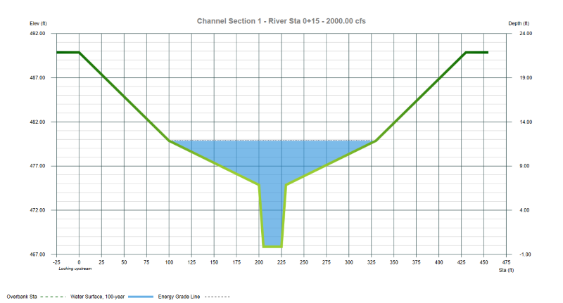
These graphs are self-explanatory. The actual channel surface corresponds to the top of the thickened green line.

You can utilize the options in the upper right of the plot for the following:
EGL
This draws the Energy Grade Line (Water Surface + Velocity Head) when turned on.
Persistent Scale
When checked on, this will use a single X, Y scale for all cross-sections. Note that if you have any cross-sections void of their geometric data, you will see a blank screen. Either turn this function off or add the remaining data.
Moving the Section Centerline
The software automatically sets the centerline of each section at it’s midpoint and aligns this with the Reach. So when you view this on the Plan the section is centered on the Reach. You can change this location by turning the CL checkbox On and exposing the centerline. Then you can simple drag the CL line with your mouse to a new location.
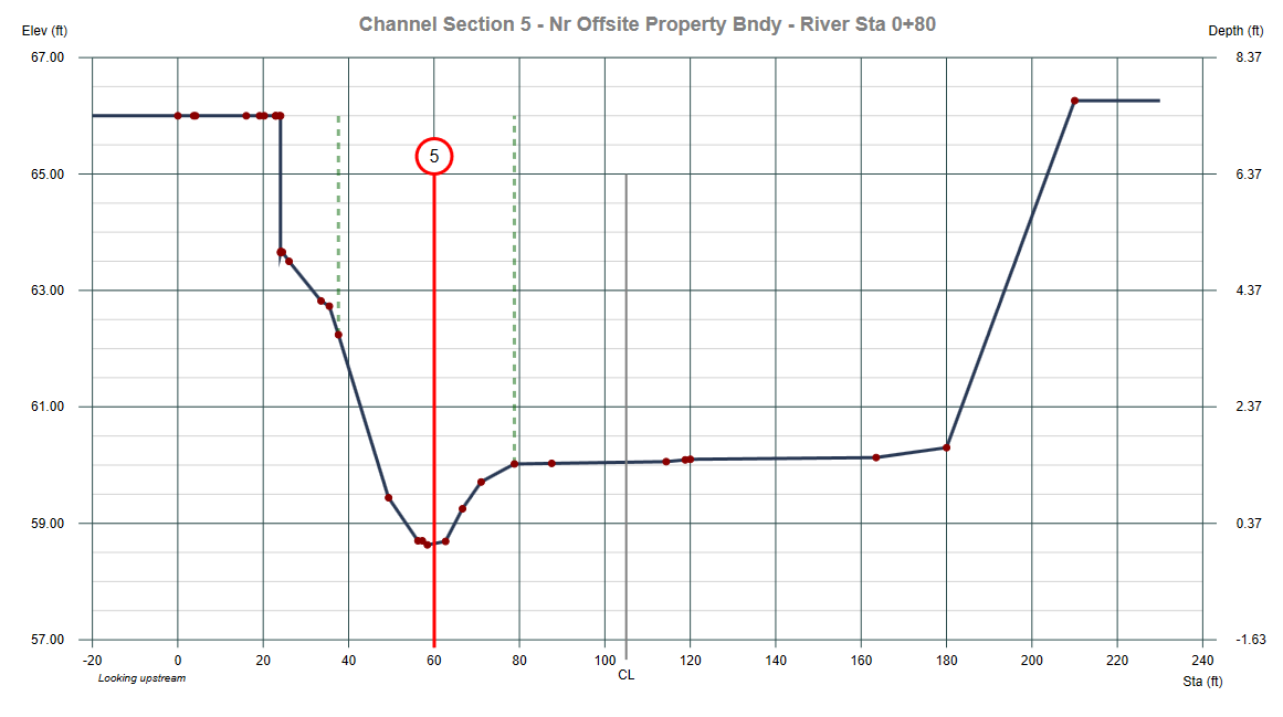
In the section above, the CL was set originally to 105 ft (210/2). The CL line was then dragged to a new position at 60. In Plan view the entire cross-section will be shifted 45 feet to the left as looking upstream.
Note that the CL option will be disabled when connected to a TIN surface. Disengage the TIN surface to use this feature.
Getting Hard Copies
You can instantly export this graph as an image file for insertion into other documents by right-clicking anywhere on the plot and choosing, “Export this Chart…”.
Of course, a more formal presentation is available by clicking on the [Print] button on the top Ribbon Menu, Home tab. See Printing Results for more information.